Python / Matlab Example
Note that this instruction is written for the Python example. The Matlab example works analogously.
Design rationale
The design of the project templates is guided by the following main thoughts:
Separation of logical chunks: A minimal requirement for a project to scale.
Only execute required tasks, automatically: Again required for scalability. It means that the machine needs to know what is meant by a “required task”.
Re-use of code and data instead of copying and pasting: Else you will forget the copy & paste step at some point down the road. At best, this leads to errors; at worst, to misinterpreting the results.
Be as language-agnostic as possible: Make it easy to use the best tool for a particular task and to mix tools in a project.
Separation of inputs and outputs: Required to find your way around in a complex project.
I will not touch upon the last point until the pyorganisation section below. The remainder of this page introduces an example and a general concept of how to think about the first four points.
Running example
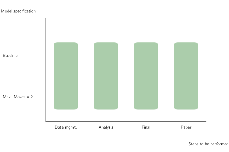
To fix ideas, let’s look at the example of Schelling’s (1969, [Sch69]) segregation model, as outlined here in Stachurski’s and Sargent’s online course [SS19]. Please look at their description of the Schelling model. Say we are thinking of two variants for the moment:
Replicate the figures from Stachurski’s and Sargent’s course.
Check what happens when agents are restricted to two random moves per period; after that they have to stop regardless whether they are happy or not.
For each of these variants (called models in the project template and the remainder of this document), you need to perform various steps:
Draw a simulated sample with initial locations (this is taken to be the same across models, partly for demonstration purposes, partly because it assures that the initial distribution is the same across both models)
Run the actual simulation
Visualise the results
Pull everything together in a paper.
It is very useful to explictly distinguish between steps 2. and 3. because computation time in 2. becomes an issue: If you just want to change the layout of a table or the color of a line in a graph, you do not want to wait for days. Not even for 3 minutes or 30 seconds as in this example.
How to organise the workflow?
A naïve way to ensure reproducibility is to have a master-script (do-file, m-file, …) that runs each file one after the other. One way to implement that for the above setup would be to have code for each step of the analysis and a loop over both models within each step:
You will still need to manually keep track of whether you need to run a particular step after making changes, though. Or you run everything at once, all the time. Alternatively, you may have code that runs one step after the other for each model:
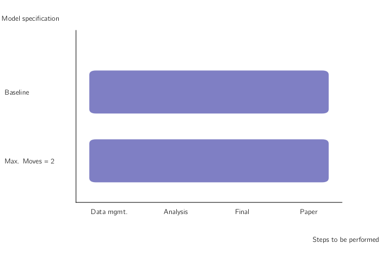
The equivalent comment applies here: Either keep track of which model needs to be run after making changes manually, or run everything at once.
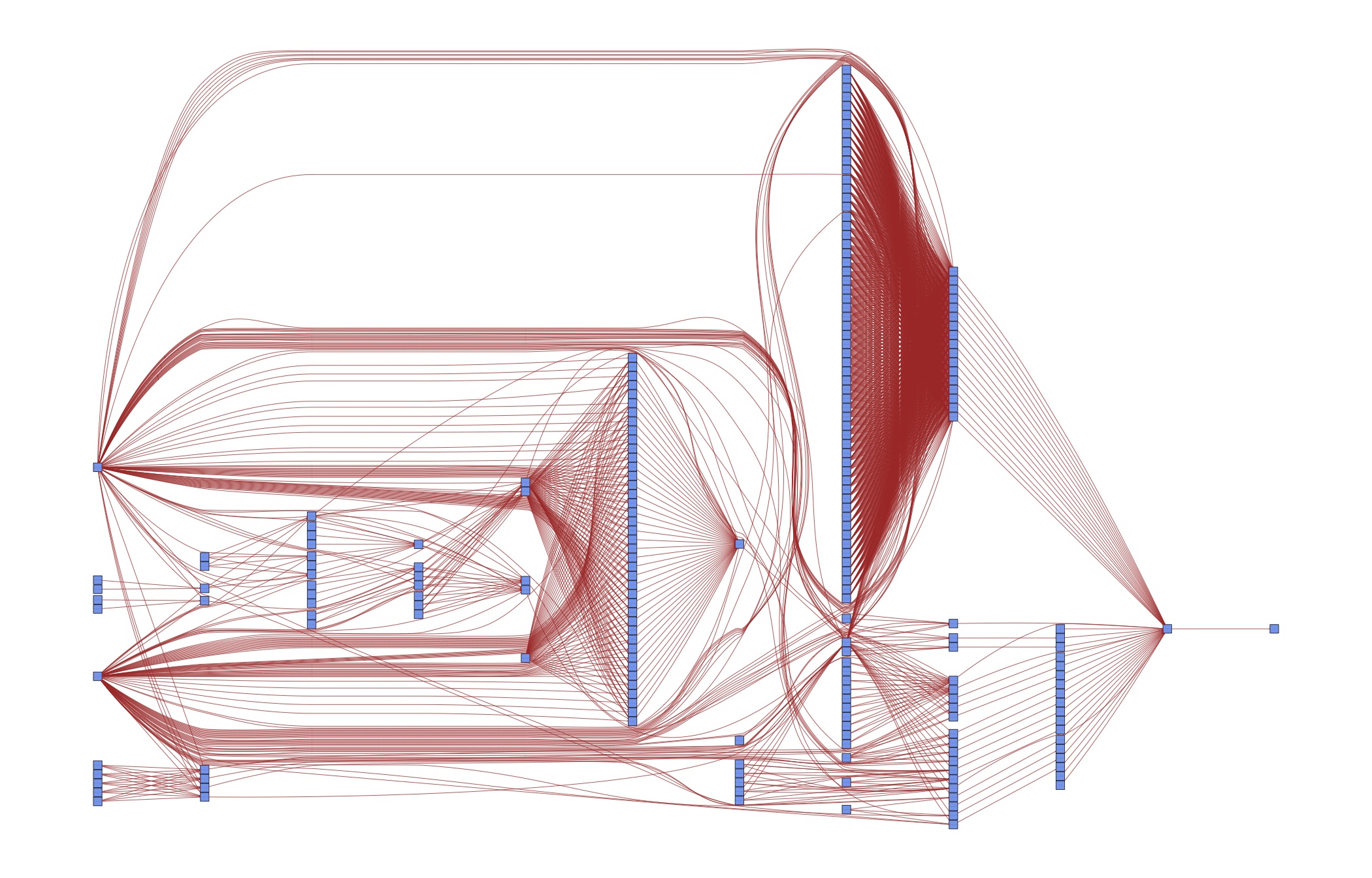
Ideally though, you want to be even more fine-grained than this and only run individual elements. This is particularly true when your entire computations take some time. In this case, running all steps every time via the master-script simply is not an option. All my research projects ended up running for a long time, no matter how simple they were… The figure shows you that even in this simple example, there are now quite a few parts to remember:
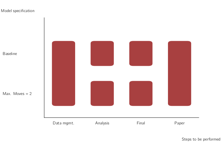
This figure assumes that your data management is being done for all models at once, which is usually a good choice for me. Even with only two models, we need to remember 6 ways to start different programs and how the different tasks depend on each other. This does not scale to serious projects!
Directed Acyclic Graphs (DAGs)
The way to specify dependencies between data, code and tasks to perform for a computer is a directed acyclic graph. A graph is simply a set of nodes (files, in our case) and edges that connect pairs of nodes (tasks to perform). Directed means that the order of how we connect a pair of nodes matters, we thus add arrows to all edges. Acyclic means that there are no directed cycles: When you traverse a graph in the direction of the arrows, there may not be a way to end up at the same node again.
This is the dependency graph for the modified Schelling example from Stachurski and Sargent, as implemented in the Python branch of the project template:
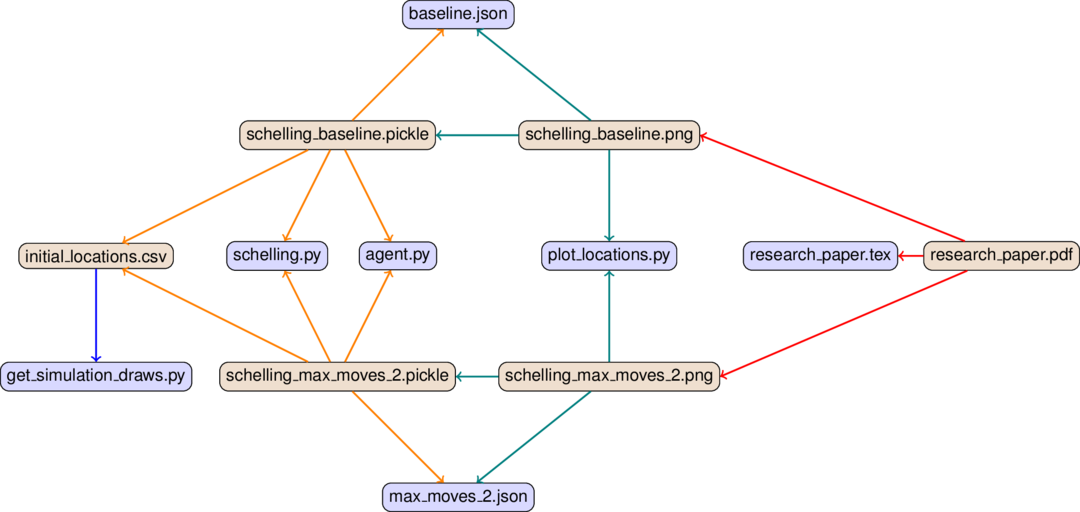
The arrows have different colors in order to distinguish the steps of the analysis, from left to right:
Blue for data management (=drawing a simulated sample, in this case)
Orange for the main simulation
Teal for the visualisation of results
Red for compiling the pdf of the paper
Bluish nodes are pure source files – they do not depend on any other file and hence none of the edges originates from any of them. In contrast, brownish nodes are targets, they are generated by the code. Some may serve as intermediate targets only – e.g. there is not much you would want to do with the raw simulated sample (initial_locations.csv) except for processing it further.
In a first run, all targets have to be generated, of course. In later runs, a target only needs to be re-generated if one of its direct dependencies changes. E.g. when we make changes to baseline.json, we will need to build schelling_baseline.pickle and schelling_baseline.png anew. Depending on whether schelling_baseline.png actually changes, we need to re-compile the pdf as well. We will dissect this example in more detail in the next section. The only important thing at this point is to understand the general idea.
Of course this is overkill for a textbook example – we could easily keep the code closer together than this. But such a strategy does not scale to serious papers with many different specifications. As a case in point, consider the DAG for an early version of [vG15]:
Do you want to keep those dependencies in your head? Or would it be useful to specify them once and for all in order to have more time for thinking about research? The next section shows you how to do that.
Introduction to pytask
pytask is our tool of choice to automate the dependency tracking via a DAG (directed acyclic graph) structure. It has been written by Uni Bonn alumnus Tobias Raabe out of frustration with other tools.
pytask is inspired by pytest and leverages the same plugin system. If you are familiar with pytest, getting started with pytask should be a very smooth process.
pytask will look for Python scripts named task_[specifier].py in all subdirectories of your project. Within those scripts, it will execute functions that start with task_.
Have a look at its excellent documentation. At present, there are additional plugins to run R scripts, Stata do-files, and to compile documents via LaTeX.
We will have more to say about the directory structure in the pyorganisation section. For now, we note that a step towards achieving the goal of clearly separating inputs and outputs is that we specify a separate build directory. All output files go there (including intermediate output), it is never kept under version control, and it can be safely removed – everything in it will be reconstructed automatically the next time you run pytask.
Pytask Overview
From a high-level perspective, pytask works in the following way:
pytask reads your instructions and sets the build order.
Think of a dependency graph here.
It stops when it detects a circular dependency or ambiguous ways to build a target.
Both are major advantages over a master-script, let alone doing the dependency tracking in your mind.
pytask decides which tasks need to be executed and performs the required actions.
Minimal rebuilds are a huge speed gain compared to a master-script.
These gains are large enough to make projects break or succeed.
We have just touched upon the tip of the iceberg here; pytask has many more goodies to offer. Its documentation is an excellent source.
Wanted: Feedback
This is very fresh; please let us know what you would like to see here and what needs better explanation.
Organisation
On this page, we describe how the files are distributed in the directory hierarchy.
Directory structure
[The pictures are a little outdated, but you get the idea]
The left node of the following graph shows the contents of the project root directory after executing pytask:
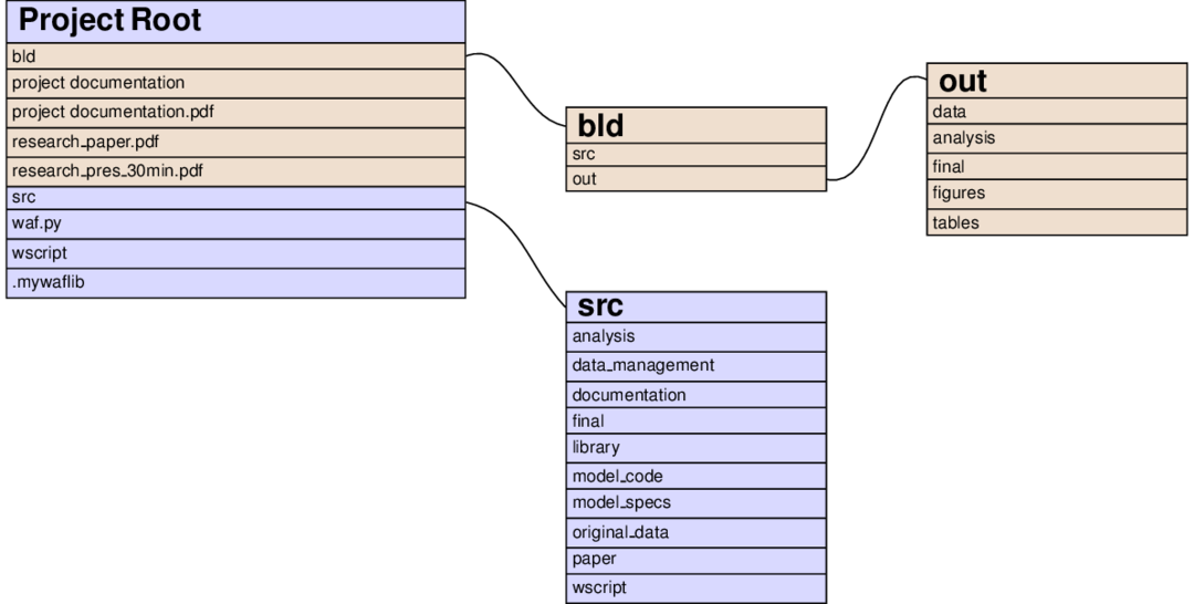
Files and directories in brownish colours are constructed by pytask; those with a bluish background are added directly by the researcher. You immediately see the separation of inputs and outputs (one of our guiding principles) at work:
All source code is in the src directory.
All outputs are constructed in the bld directory.
The paper and presentation are put there so they can be opened easily.
The contents of both the root/bld and the root/src directories directly follow the steps of the analysis from the workflow section.
The idea is that everything that needs to be run during the, say, analysis step, is specified in root/src/analysis and all its output is placed in root/bld/analysis.
Some differences:
Because they are accessed frequently, figures and tables get extra directories in root/bld
The directory root/src contains many more subdirectories:
original_data is the place to store the data in its raw form, as downloaded / transcribed / … The original data should never be modified and saved under the same name.
model_code contains source files that might differ by model and that are potentially used at various steps of the analysis.
model_specs contains JSON files with model specifications. The choice of JSON is motivated by the attempt to be language-agnostic: JSON is quite expressive and there are parsers for nearly all languages (for Stata there is a converter in root/src/model_specs/task_models.py file of the Stata version of the template)
library provides code that may be used by different steps of the analysis. Little code snippets for input / output or stuff that is not directly related to the model would go here. The distinction from the model_code directory is a bit arbitrary, but I have found it useful in the past.
As an example of how things look further down in the hierarchy, consider the analysis step:
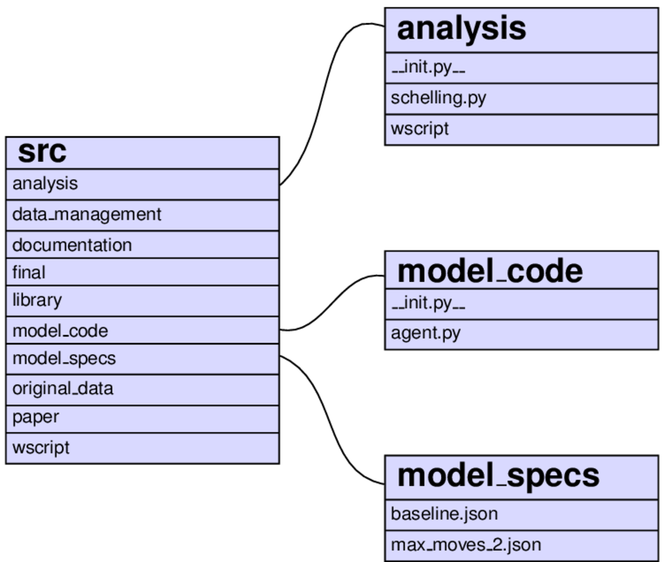
The same function (task_schelling) is run twice for the models baseline and max_moves_2. All specification of files is done in pytask.
It is imperative that you do all the task handling inside the task_xxx.py-scripts, using the pathlib library. This ensures that your project can be used on different machines and it minimises the potential for cross-platform errors.
For running Python source code from pytask, simply include depends_on and produces as inputs to your function.
For running scripts in other languages, pass all required files (inputs, log files, outputs) as arguments to the @pytask.mark.[x]-decorator. You can then read them in. Check the other templates for examples.